Abstract:
FINAL REPORT - PERSONAL SAVINGS
Aaron Koga
Econ 425
11 December 2006
Introduction
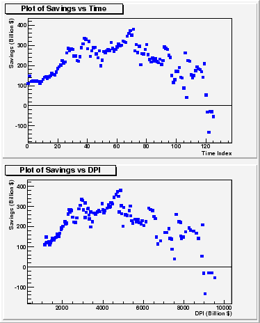
Recently in America, personal savings has rapidly decreased. Savings is important because it provides future consumption for individuals as well as resources for investment in the nation as a whole.
Traditionally, the biggest factor in determing personal savings is disposable personal income (DPI).
The portion of DPI which is saved is known as the personal savings rate.
However, the recent decline in personal savings cannot be explained by changes in DPI alone.
Thus, additional factors such as increases in wealth due to rapid rises in housing prices
have been suggested to explain this discrepancy ![]() .
.
Fitting and Interpretation
Personal Savings vs DPI
|
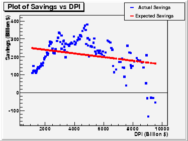
A regression of the personal savings on DPI using the equation
yielded the results listed in TABLE I and displayed in FIG 2. Although the fit is significant according to the F-statistic, as the low
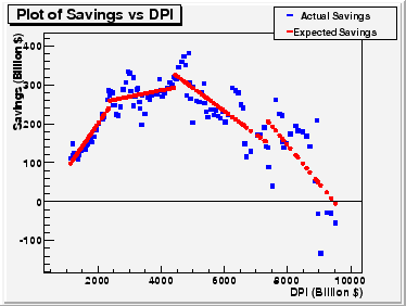
In 1982, America experienced a serious recession. As the data suggests, this recession probably had an impact on the savings rate. This type of assumption can be logically justified. During recessions people often experience hardships such as the loss of jobs. Due to these new budjet constraints, people are forced to change their spending and saving habits. After keeping these new habits for a certain period of time, people become used to them and when the recession eventually ends, they persist in their new habits. In addition to the 1982 recession, there may also have been effects from the 1991 and 2001 recessions on the savings rate.
To account for the changes in the savings rate due to the recessions, dummy variables (![]() ) were used
to form the following equation:
) were used
to form the following equation:
| (2) |
where
As can be seen from FIG 3 and the increased
![]() , (2) is an improvement over (1).
Testing
, (2) is an improvement over (1).
Testing ![]() (i=1,2,3 j=0,1), yielded an F-value of 51.2558.
Thus, allowing for changes in the savings rate during each period of recession seems justified.
This can also be seen in the significance of the t-values for the coefficients
(i=1,2,3 j=0,1), yielded an F-value of 51.2558.
Thus, allowing for changes in the savings rate during each period of recession seems justified.
This can also be seen in the significance of the t-values for the coefficients ![]() in TABLE II.
This fit says that while 12 cents was saved for every dollar of DPI before 1982,
during and after the 1982 recession only 2 cents was saved for every dollar of DPI.
In addition, the savings rate became negative after 1991.
in TABLE II.
This fit says that while 12 cents was saved for every dollar of DPI before 1982,
during and after the 1982 recession only 2 cents was saved for every dollar of DPI.
In addition, the savings rate became negative after 1991.
Including HPI
|
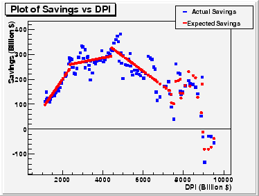
To account for the recent negative personal savings, the HPI was taken into account. As suggested by others, the increase in housing prices may help to explain the recent decrease in personal savings. Personal savings was regressed on DPI and the HPI (only since 2001, to simulate a 'recent effect') according to the equation
| (3) |
where
The increase in
![]() for (3) compared with (2) suggests
that taking into account the HPI is justified.
Also, as can be seen from the t-values and F-statistic in TABLE III, all coefficients are significant.
The fit to the data for (3), like (2), says that
while the 12 cents was saved for every dollar of DPI before 1982,
during and after the 1982 recession only 2 cents was saved for every dollar of DPI.
In addition, -6 cents was saved for every dollar of DPI
for the period 1991-2001, and 58 cents was saved for every dollar of DPI after 2001.
Also, as is expected, the negative value of
for (3) compared with (2) suggests
that taking into account the HPI is justified.
Also, as can be seen from the t-values and F-statistic in TABLE III, all coefficients are significant.
The fit to the data for (3), like (2), says that
while the 12 cents was saved for every dollar of DPI before 1982,
during and after the 1982 recession only 2 cents was saved for every dollar of DPI.
In addition, -6 cents was saved for every dollar of DPI
for the period 1991-2001, and 58 cents was saved for every dollar of DPI after 2001.
Also, as is expected, the negative value of ![]() indicates that
increases in housing prices decreases personal savings.
indicates that
increases in housing prices decreases personal savings.
Other regressions using the periods 1982-1990, 1991-200, and 2001-2006 as the base period
were run. In each regression the coefficients ![]() corresponding to terms outside
of the base year had significant t-values (see TABLE IV).
So, each period (1975-1981, 1982-1990, 1991-200, and 2001-2006) has savings rates which are
significantly different from one another.
Thus, allowing for changes in the savings rate during each period of recession, as specified,
is justified.
Also, the insignificance of
corresponding to terms outside
of the base year had significant t-values (see TABLE IV).
So, each period (1975-1981, 1982-1990, 1991-200, and 2001-2006) has savings rates which are
significantly different from one another.
Thus, allowing for changes in the savings rate during each period of recession, as specified,
is justified.
Also, the insignificance of ![]() when running the regression with 1982-1990 as the base period
suggests that the savings rate during that period of time was not significantly different from zero.
when running the regression with 1982-1990 as the base period
suggests that the savings rate during that period of time was not significantly different from zero.
|
Summary
It is apparent that when examining the personal savings rate, the effects of recessions on people's saving habits is important. Also, to explain the recent and rapid decrease in personal savings, taking into account housing prices (or potentially other types of wealth) is also important. Taking housing prices into account indicates that recent decreases in personal savings is at least partially justified.
On the other hand, a savings rate of 0.58 for the period 2001-2006 as suggested by this regression is too high to be believable. However, adding other variables to the model such as stock prices may prove useful.
References
[1] Garner, Alan. Should the Decline in the Personal Saving Rate Be a Cause for Conern. www.kc.frb.org/publicat/econrev/PDF/2Q06garn.pdf (2006).
[2] Data can be found at: http://research.stlouisfed.org/fred2/.
[3] Data can be found at: http://www.ofheo.gov/HPI.asp.
| Date | Personal Savings | HPI | DPI |
| (M/D/Y) | (Billion Dollars) | (Billion Dollars) | |
| 1/1/1975 | 110.5 | 61.63 | 1126 |
| 4/1/1975 | 148.6 | 62.97 | 1193.2 |
| 7/1/1975 | 120 | 62.32 | 1199.1 |
| 10/1/1975 | 123.2 | 63.27 | 1231.5 |
| 1/1/1976 | 121.7 | 64.38 | 1263.5 |
| 4/1/1976 | 122.9 | 66.29 | 1284.5 |
| 7/1/1976 | 124.4 | 66.82 | 1315.8 |
| 10/1/1976 | 120.2 | 68.1 | 1346.1 |
| 1/1/1977 | 109.8 | 70.09 | 1372.5 |
| 4/1/1977 | 119.5 | 72.81 | 1411.3 |
| 7/1/1977 | 130.3 | 74.71 | 1454.3 |
| 10/1/1977 | 141.4 | 77.14 | 1504.6 |
| 1/1/1978 | 144 | 79.57 | 1538.9 |
| 4/1/1978 | 134.8 | 82.41 | 1589 |
| 7/1/1978 | 143.8 | 84.94 | 1630.5 |
| 10/1/1978 | 147.5 | 87.51 | 1674.8 |
| 1/1/1979 | 162 | 91.41 | 1725.8 |
| 4/1/1979 | 154.6 | 93.99 | 1760.2 |
| 7/1/1979 | 152.6 | 96.02 | 1813.9 |
| 10/1/1979 | 167.4 | 97.91 | 1874.2 |
| 1/1/1980 | 184.9 | 100 | 1944 |
| 4/1/1980 | 194 | 101.06 | 1955.2 |
| 7/1/1980 | 201.6 | 104.27 | 2021.2 |
| 10/1/1980 | 225.4 | 104.65 | 2115.5 |
| 1/1/1981 | 211.6 | 105.77 | 2161.9 |
| 4/1/1981 | 218.3 | 107.83 | 2202.8 |
| 7/1/1981 | 262.2 | 109.25 | 2289.6 |
| 10/1/1981 | 285.1 | 109.63 | 2330.1 |
| 1/1/1982 | 273.1 | 110.97 | 2359.7 |
| 4/1/1982 | 282.7 | 111.54 | 2399.1 |
| 7/1/1982 | 280.1 | 111.09 | 2447.2 |
| 10/1/1982 | 247.2 | 112.03 | 2478.7 |
| 1/1/1983 | 247.2 | 114.02 | 2521.2 |
| 4/1/1983 | 223.3 | 115.24 | 2564.3 |
| 7/1/1983 | 220.6 | 116.07 | 2635.1 |
| 10/1/1983 | 243.3 | 116.54 | 2712.9 |
| 1/1/1984 | 288.2 | 118.24 | 2805.3 |
| 4/1/1984 | 306.5 | 120.28 | 2885.4 |
| 7/1/1984 | 334.5 | 121.44 | 2955 |
| 10/1/1984 | 330 | 122.77 | 3002.4 |
| 1/1/1985 | 283.7 | 124.57 | 3032.2 |
| 4/1/1985 | 318.9 | 126.63 | 3117.5 |
| 7/1/1985 | 245.7 | 129 | 3115.4 |
| 10/1/1985 | 271.8 | 130.77 | 3172.2 |
| 1/1/1986 | 287.7 | 133.33 | 3233.4 |
| 4/1/1986 | 290.5 | 136.27 | 3269.1 |
| 7/1/1986 | 256.4 | 138.86 | 3307.2 |
| 10/1/1986 | 238.9 | 141.42 | 3330.7 |
| 1/1/1987 | 273 | 144.55 | 3397.1 |
| 4/1/1987 | 198.1 | 147.29 | 3389.4 |
| 7/1/1987 | 225.6 | 149.63 | 3484.5 |
| 10/1/1987 | 268.7 | 151.01 | 3562.1 |
| 1/1/1988 | 262.4 | 153.71 | 3638.5 |
| 4/1/1988 | 273.7 | 156.97 | 3711.3 |
| 7/1/1988 | 280 | 158.68 | 3786.9 |
| 10/1/1988 | 275.5 | 160.36 | 3858.2 |
| 1/1/1989 | 314 | 162.48 | 3954.9 |
| 4/1/1989 | 285.3 | 164.65 | 3993.4 |
| 7/1/1989 | 269.7 | 168.45 | 4038.8 |
| 10/1/1989 | 279.5 | 170.04 | 4099.5 |
| 1/1/1990 | 292.6 | 170.73 | 4198.2 |
| 4/1/1990 | 307.2 | 170.68 | 4268.1 |
| 7/1/1990 | 297.8 | 171.28 | 4325.7 |
| 10/1/1990 | 300 | 170.48 | 4351.3 |
| 1/1/1991 | 320.4 | 171.78 | 4387.1 |
| 4/1/1991 | 317.7 | 172.56 | 4441.8 |
| 7/1/1991 | 313.7 | 172.54 | 4483.7 |
| 10/1/1991 | 344.7 | 174.9 | 4544.5 |
| 1/1/1992 | 359.4 | 176.05 | 4651.4 |
| 4/1/1992 | 373.8 | 175.68 | 4716.1 |
| 7/1/1992 | 350.1 | 177.45 | 4768.6 |
| 10/1/1992 | 380.9 | 178.19 | 4869.6 |
| 1/1/1993 | 272.4 | 177.92 | 4801.6 |
| 4/1/1993 | 304.3 | 179.4 | 4901.1 |
| 7/1/1993 | 264.5 | 180.49 | 4924.3 |
| 10/1/1993 | 295.1 | 181.88 | 5020.8 |
| 1/1/1994 | 203.3 | 182.73 | 4998.7 |
| 4/1/1994 | 258.8 | 183.34 | 5118.1 |
| 7/1/1994 | 256.3 | 183.84 | 5197.5 |
| 10/1/1994 | 279.4 | 183.39 | 5293.1 |
| 1/1/1995 | 302.9 | 184.07 | 5350.9 |
| 4/1/1995 | 253 | 187.28 | 5376.3 |
| 7/1/1995 | 230.3 | 190.19 | 5427.1 |
| 10/1/1995 | 217.6 | 191.69 | 5478.6 |
| 1/1/1996 | 236.5 | 194.03 | 5574.5 |
| 4/1/1996 | 223 | 194.22 | 5656.6 |
| 7/1/1996 | 234.9 | 194.97 | 5727.5 |
| 10/1/1996 | 219.2 | 196.64 | 5795.3 |
| 1/1/1997 | 213.7 | 198.44 | 5877.4 |
| 4/1/1997 | 230.6 | 200.05 | 5936.7 |
| 7/1/1997 | 204.7 | 203 | 6020.8 |
| 10/1/1997 | 224.3 | 205.66 | 6120.5 |
| 1/1/1998 | 291.7 | 208.8 | 6255.9 |
| 4/1/1998 | 285.4 | 210.44 | 6357.7 |
| 7/1/1998 | 280.5 | 213.34 | 6448.1 |
| 10/1/1998 | 249.6 | 215.9 | 6522.1 |
| 1/1/1999 | 240.4 | 218.09 | 6586.7 |
| 4/1/1999 | 149.1 | 221.04 | 6638.6 |
| 7/1/1999 | 115 | 224.45 | 6708.2 |
| 10/1/1999 | 129.7 | 226.96 | 6846.2 |
| 1/1/2000 | 171.2 | 231.67 | 7059.2 |
| 4/1/2000 | 171.3 | 235.58 | 7141.2 |
| 7/1/2000 | 190.1 | 240.15 | 7266.4 |
| 10/1/2000 | 141.2 | 244.1 | 7309.3 |
| 1/1/2001 | 138.6 | 250.41 | 7392.1 |
| 4/1/2001 | 88.7 | 254.87 | 7407.6 |
| 7/1/2001 | 261.6 | 259.1 | 7622.8 |
| 10/1/2001 | 40.5 | 262.48 | 7524.8 |
| 1/1/2002 | 225.4 | 266.74 | 7751.5 |
| 4/1/2002 | 221.2 | 271.73 | 7841.7 |
| 7/1/2002 | 153 | 277.59 | 7845.4 |
| 10/1/2002 | 139.3 | 281.97 | 7881.7 |
| 1/1/2003 | 149.1 | 285.71 | 7975.5 |
| 4/1/2003 | 173.9 | 289.29 | 8087.6 |
| 7/1/2003 | 194 | 294.2 | 8261 |
| 10/1/2003 | 182.5 | 304.06 | 8326 |
| 1/1/2004 | 178.9 | 309.24 | 8481.6 |
| 4/1/2004 | 168.3 | 317.77 | 8607.1 |
| 7/1/2004 | 141.2 | 331.97 | 8706.3 |
| 10/1/2004 | 208.9 | 340.29 | 8931.2 |
| 1/1/2005 | 52.5 | 349.61 | 8890.9 |
| 4/1/2005 | -30.8 | 362.38 | 8969.7 |
| 7/1/2005 | -132.6 | 374.23 | 9047.7 |
| 10/1/2005 | -28.5 | 385.76 | 9236.1 |
| 1/1/2006 | -29.7 | 394.23 | 9388.8 |
| 4/1/2006 | -54.6 | 398.85 | 9522.4 |