Abstract:
This paper draws an analogy between a system in thermal and diffusive contact with a reservoir and
financial markets.
As a result of this analogy, a chemical potential can be defined for the markets.
It seems that the moving average of the chemical potential, when averaged over an appropriate window of time,
may reach a peak around market bottoms.
This is most successfully demonstrated for the 2002 market bottom.
The chemical potential of a few individual stocks is also examined.
CHEMICAL POTENTIAL OF THE STOCK MARKET
Aaron Koga
4 May 2007
Introduction
Much effort has been expended in the study of financial markets. Many different models have been developed to predict future price changes in the market based on recent trends. Although the effectiveness of technical analysis is consistently disputed by academic studies, there have been countless man hours invested in the creation of various statistical models for financial markets. In recent years, various models and mathematics, typically used in the description of physical systems, have been applied to financial markets.
For example, a paper last year by Kleinert and Chen fitted price changes in the S&P500 and NASDAQ 100 to a Boltzmann distribution. Normally used in statistical mechanics, this distribution was used to describe the short term price changes of the markets. Kleinert and Chen showed that the distribution widens as a function of the sampling period, as theory predicts. Also, they demonstrated that the ``temperature'' of the market (a parameter in the Boltzmann distribution) reached a maximum as the market peaked in 2001 [1].
In another study, a group of professors at the University of Tokyo showed that the S&P500 exhibited ``critical'' behavior surrounding the 1987 market crash known as Black Monday. They found that although the variance of the probability density function of price changes in the market normally scales with time, this behavior breaks down near market crashes. This is in analogy to the behavior of spins in a ferromagnetic material as the material reaches its critical temperature [2].
This paper draws an analogy between markets and a system-reservoir model in thermodynamics; the parameter known as the chemical potential is then examined for the market.
System-Reservoir Model
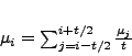
The chemical potential, ![]() , in thermodynamics is defined as
, in thermodynamics is defined as
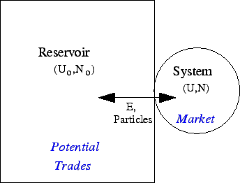
An analogy can be drawn between the system-reservoir model and financial markets. Suppose that a financial market in a given period of time is a system with N particles and energy U. In that period of time, there are a number of trades executed and a price change in the market. Thus, it is intuitive to say that each trade is a particle in the system of the market. In a physical system, each particle may contribute to the energy. Likewise, each trade in the market contributes to the total increase or decrease in the price of the market. The energy is thus the equivalent of relative price change (percent change) in the market.
Only a certain number of trades are made in the market (the system) during a period of time. However, the potential number of trades is much greater. If everyone who owns shares of a stock or who could buy shares of a stock attempted to trade in the market, a very large number of trades would be made with a finite change in market price. This system of potential trades, because it is so big, can be thought of as a reservoir.
The number of trades executed, ![]() , and resulting relative price change,
, and resulting relative price change, ![]() , varies from time period to time period.
This can be thought of as a flow of particles and energy between the reservoir and the system.
Thus, the quantity known as the chemical potential,
, varies from time period to time period.
This can be thought of as a flow of particles and energy between the reservoir and the system.
Thus, the quantity known as the chemical potential,
Measuring Chemical Potential
A graphing program known as Root, which is a C-interpreter,
was used to calculate and examine ![]() of the market.
A Root script, PLOT
of the market.
A Root script, PLOT![]() pot
pot![]() A.cpp, was written to
find the chemical potential from a file of historical data, obtained at
finance.yahoo.com.
The most frequently sampled data (daily data) was used.
A.cpp, was written to
find the chemical potential from a file of historical data, obtained at
finance.yahoo.com.
The most frequently sampled data (daily data) was used.
Chemical Potential of a Day
The ![]() of day
of day ![]() was calculated as
was calculated as

Chemical Potential Moving Average
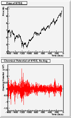
This method for calculating the chemical potential was applied to data for the New York Stock Exchange (NYSE).
The results, plotted in FIG 2, are very noisy and difficult to interpret.
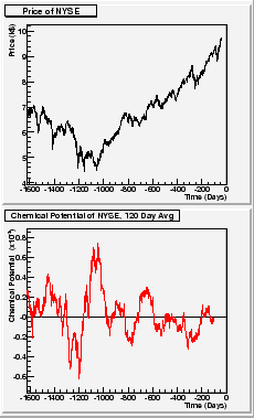
To average out some of the noise, a simple moving average was taken of the chemical potential.
The equation
Chemical Potential of Various Indices
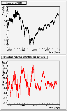
The 120 day moving average was found for the Dow Jones Industrial Average (DJIA), NASDAQ, and S&P500. These are plotted in FIG 4-6.
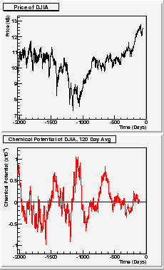
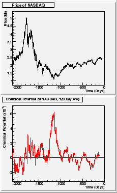
Of the indices examined here, the NASDAQ (the technology index that was hardest hit by the bear market) shows the clearest peak in chemical potential at the bottom of the 2002 bear market. Other local peaks in
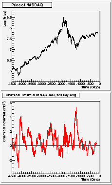
More history for the NASDAQ was examined and the results are plotted in FIG 7.
While it seems that the largest peaks in ![]() correspond to market bottoms,
smaller peaks in
correspond to market bottoms,
smaller peaks in ![]() do not show a consistent correspondence
do not show a consistent correspondence
 |
Chemical Potential of Individual Stocks
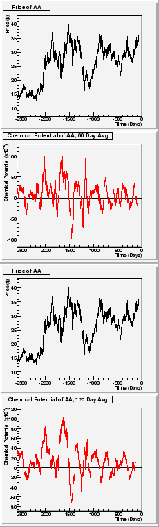
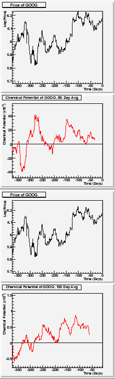
 -moving average, Time=0 corresponds to most recent day (April 2007). 60-day moving average (Top) is a better fit than the 120-day moving average (Bottom).
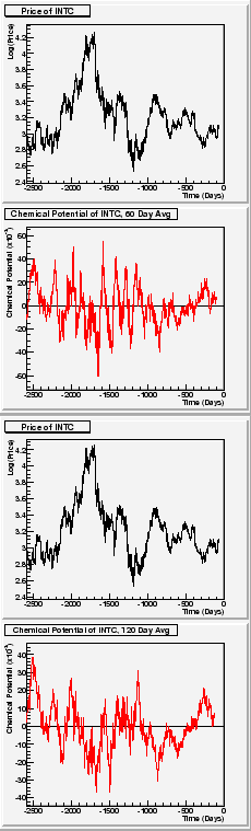 -moving average, Time=0 corresponds to most recent day (April 2007). 120-day moving average (Bottom) is a better fit than the 60-day moving average (Top).
In addition to the chemical potential of market indices, the potential of individual stocks was also examined.
Tuning of the parameter ![]() was necessary to obtain a good potential.
The chemical potential for Alcoa, shown in FIG 8 was found with
was necessary to obtain a good potential.
The chemical potential for Alcoa, shown in FIG 8 was found with ![]() optimized to 60 days.
On the other hand, the potential for Intel, shown in FIG 9,
was found with
optimized to 60 days.
On the other hand, the potential for Intel, shown in FIG 9,
was found with ![]() optimized to
120 days.
While Alcoa has daily volume on the order of 5-10 million shares,
Intel has daily volume on the order of 50-100 million shares.
Thus, it was postulated that
optimized to
120 days.
While Alcoa has daily volume on the order of 5-10 million shares,
Intel has daily volume on the order of 50-100 million shares.
Thus, it was postulated that ![]() of larger stocks (and market indices) need to be averaged over
larger periods of time than the
of larger stocks (and market indices) need to be averaged over
larger periods of time than the ![]() of smaller stocks.
of smaller stocks.
To further explore this, two other companies, Google (FIG 10) and Dell (FIG 11)
were examined.
Google, which has daily volume on the same order as Alcoa, was better suited
to a ![]() of 60 days.
On the other hand, Dell, which has daily volume on the same order as Intel, was better suited to a
of 60 days.
On the other hand, Dell, which has daily volume on the same order as Intel, was better suited to a ![]() of 120 days.
This seemed to confirm that larger stocks should be averaged over longer periods of time.
of 120 days.
This seemed to confirm that larger stocks should be averaged over longer periods of time.
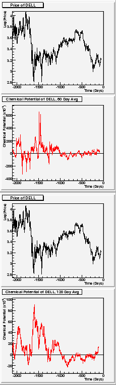 -moving average, Time=0 corresponds to most recent day (April 2007). 120-day moving average (Bottom) is a better fit than the 60-day moving average (Top).
Conclusions
The market can be thought of as a system that is in thermal and diffusive contact with a reservoir. It is then possible to define a chemical potential for the market and show that it has a significant peak during the market bottom of 2002. While significant potential peaks may correspond with market bottoms, smaller potential peaks do not have this correspondence. Also, minimum values of the potential do not consistently correspond with market tops.
In technical analysis, the term ``follow through'' refers to days coming out of a correction when the market advances on higher volume. These days are thought to signal a healthy recovery for the market and often occur with only slightly higher volume. In addition, market advances on increasing volume accompanied by market declines on decreasing volume are thought to be a bullish sign. The correspondence of peaks in the chemical potential with market bottoms may be a manifestation of these two beliefs.
Market tops are often thought to occur with large advances as well as declines. Declines are often met with increasing volume. Advances, however, are sometimes met with increasing and sometimes with decreasing volume. If this happens, then the chemical potential would not exhibit any real correspondence with market tops.
When examining the chemical potential of individual stocks, there seems to be a correlation between
market bottoms and peaks in the potential.
It is important, however, to apply the correct ![]() to find the moving average;
to find the moving average;
![]() tends to be larger for stocks with larger volume.
The differences in optimal
tends to be larger for stocks with larger volume.
The differences in optimal ![]() may reflect the tendency for smaller stocks to
react more vigorously to changing expectations and developments in the company.
may reflect the tendency for smaller stocks to
react more vigorously to changing expectations and developments in the company.
The chemical potential, given in EQ 1, assumes that the entropy and volume of the system remain constant. However, these quantities are not defined for the market. Thus, attempts to quantify them may prove useful.
Even if one believes the relationship between the chemical potential and market prices presented in this paper, because moving averages are necessary to detect market bottoms, by the time a peak in the chemical potential is observed, the market will already have reached a bottom.
Bibliography
-
- 1
- H. Kleinert and X.J. Chen, Boltzmann Distribution and Temperature of Stock Markets, arXiv:physics/0609209v2, (2006).
- 2
- Y. Yamamoto, K. Kiyono, Z.R. Struzik, Critically and Phase Transition in Stock-Price Fluctuations, Phys. Rev. Lett. 96, 068701 (2006).
- 3
- C. Kittel and H. Kroemer, Thermal Physics, 2nd Edition, Twenty-fourth Printing (1980).
- 4
- Financial Market, http://en.wikipedia.org/wiki/Financial
 market.
- 5
- Find data at finance.yahoo.com.