Aaron Koga
Physics 305
24 April 2007
Introduction
Objects in space exert gravitational forces on each other.
The force exerted on body 1 by body 2 is given by
This lab studied the Earth-moon orbit and the Apollo 13 mission with computer simulations.
Earth-Moon Orbit
Earth-Moon C Program
A C Program, earth
Basically, the program passes functions for the position and velocity derivatives for the
Earth and the moon (f![]() rE(), f
rE(), f![]() vE(), f
vE(), f![]() rM(), f
rM(), f![]() vM()) to the RK4 function, which performs
the calculations for integration.
The derivative equations are governed by the gravitational force, given in EQ 1.
vM()) to the RK4 function, which performs
the calculations for integration.
The derivative equations are governed by the gravitational force, given in EQ 1.
Earth-Moon Results
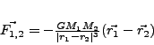
The results of a simulation for the orbit of the moon around the Earth are shown in FIG 1. As expected, the moon goes in a circular orbit around the Earth. The Earth barely moves during the orbit because its mass is large compared to the moon.
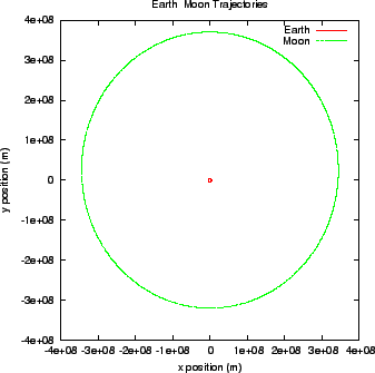
The RK4 method performs calculation for the change in position and velocity of the moving bodies at finite time intervals. This time step was varied and the relationship between the energy lost during one orbit and the time step is shown in FIG 2. The energy loss is 0.1% for a time step of about 2000 s and 0.001% for a time step of about 2 s.
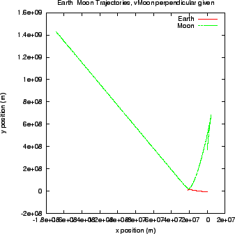
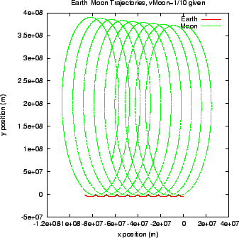
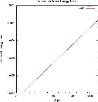
The simulation was also run for a situation where the Earth and moon had equal masses. The results, in FIG 3, show that the Earth now has a large orbit. With lower mass, the Earth is more responsive to the force on it by the moon. A run was also made with the moon having velocity perpendicular to the Earth's. The simulation was run with the moon's velocity directly away from the Earth. The results are shown in FIG 4. The moon's mass was then reduced to 1/10 the real size. The simulation of the orbit, shown in FIG 5, shows that the moon no longer orbits around the Earth. The gravitational acceleration of the moon is larger due to its smaller mass. Thus, with a normal velocity, it falls towards the Earth.
Apollo Mission
To simulate the Apollo 13 mission, earth![]() moon.c was modified.
Functions for the position and velocity derivatives of a space craft (f
moon.c was modified.
Functions for the position and velocity derivatives of a space craft (f![]() rA(), f
rA(), f![]() vA()) were added.
These functions added the forces of gravity exerted on the space craft by the Earth and the moon
to obtain the acceleration of the space craft.
These two functions were passed to the RK4 function along with the other four for the Earth and moon.
vA()) were added.
These functions added the forces of gravity exerted on the space craft by the Earth and the moon
to obtain the acceleration of the space craft.
These two functions were passed to the RK4 function along with the other four for the Earth and moon.
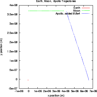
Starting from a parking orbit 185 km above the Earth's surface, Apollo 13 was instantaneously changed so that it would hit the moon. The trajectory of Apollo 13 hitting the moon is shown in FIG 6.
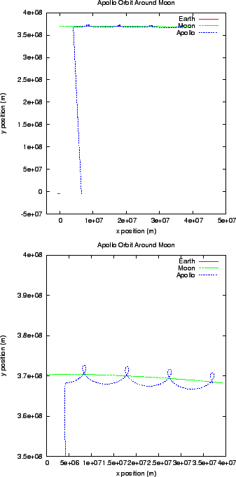
Using the same trajectory used to hit the moon, an additional change in velocity was applied to the space craft when it reached the moon. This additional change in velocity was used put the space craft into orbit around the moon. The entire flight of Apollo 13 from Earth and a few orbits around the moon are shown in FIG 7.
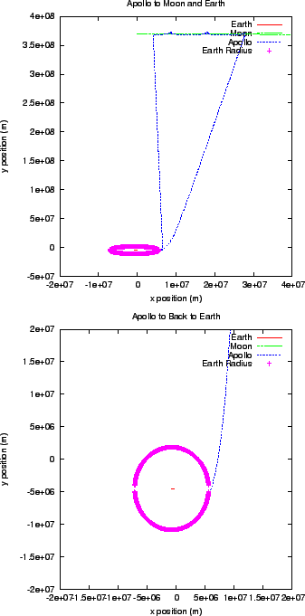
The entire trip of Apollo 13 was simulated. The trajectory for the space craft is shown in FIG 8. Adding to the conditions from the orbit of Apollo 13 around the moon (results that are shown in FIG 7), a change in velocity was made during Apollo 13's orbit around the moon. This change in velocity was made so that Apollo 13 could return to Earth. As shown in FIG 8, Apollo 13 is able to make its historic trip and return to Earth.