Aaron Koga
Physics 305
13 Feb 2007
Physics 305
13 Feb 2007
1. Introduction
Random sequences are
sequences in which there is no correlation among its members.
Because computers are deterministic, they cannot generate truly random
sequences of numbers. However, computers are often used to
simulate naturally occurring random events in processes such as Monte
Carlo simulations [1]. Computers can produce seemingly random
sequences of numbers using different techniques. To produce these
pseudo random numbers, computers have built in functions such as
drand48(), which generates a uniform distribution of numbers in the
range [0,1) using a seeded number. This lab examines computer
generated random numbers by using the computer to generate random paths
in 2 and 3 dimensions.
2. Walking a Random Path
A. C Program
C Programs were
written to use computer generated random numbers to walk 2D and 3D
paths. Because the two programs are very similar, only the
program for the 3D case is shown in the Appendix
and only the 3D program will be explained here in the text (links to
the 3D and 2D
programs). The program takes a command line input to determine
the number of paths to walk and number of steps to take in each
path. Individual
steps in each path are taken by calling the function drand48() to
determine the x, y, and z coordinates of each step. The movement
in each direction (x, y, and z) are in the range
[-sqrt(2),sqrt(2)). Because drand48() returns values in the range
[0,1), 0.5 is subtracted from the randomly generated number (to get it
into the range [-0.5, 0.5)) and then the number is multiplied by
sqrt(8). In other words,
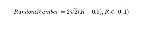 (1),
(1),
(1),where R is the number generated by
drand48(). The program also outputs files for several individual paths as
well as the average
distance walked as a function of the number of steps taken.
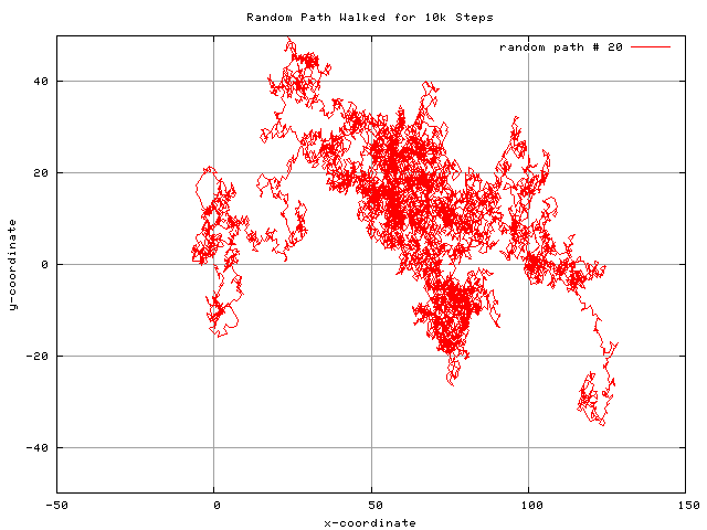
FIG1: A random 2D path with 10k steps.
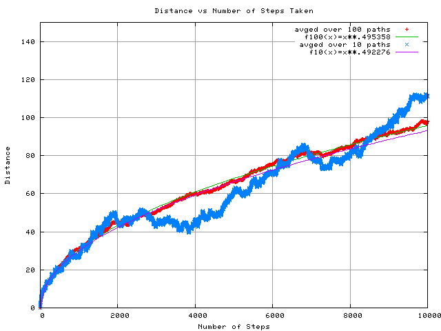
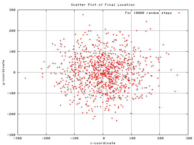
FIG3: Scatter plot of the final x-y coordinates of several
10k step paths.
B. 2D Path
FIG1: A random 2D path with 10k steps.
First, the C program
to walk a 2D path was run. One such path is displayed in
FIG1. The program was run for paths with 10k steps, with the
number of paths set to 10 and 100. The average distance, D, as a
function of the number of steps taken, N, is plotted in FIG2. The
distance, D, was fitted as a function of N to a function of the form:
D=N^(p), where p is an exponent whose value is theoretically 0.5.
As seen in FIG2, the value of p when 100 paths were taken is 0.495 and
the value of p when 10 paths were taken is 0.492. A scatter plot
of the final position (in x-y space) is shown in FIG3 for a path
consisting of 10k steps.
FIG2: Plot of the average distance versus the number of steps taken for a 10k step path. The distance is averaged over 10 paths (blue) and 100 paths (red). The average distance is also fitted as a function of the number of steps; for the 100 step path: D=N^(.495), and for the 10 step path: D=N^(.492).
FIG3: Scatter plot of the final x-y coordinates of several
10k step paths.
The program was also
run for a case where 4 paths were taken, each with 1000 steps. D
versus N for this case is plotted in FIG4. In this case p was
found to be 0.518.
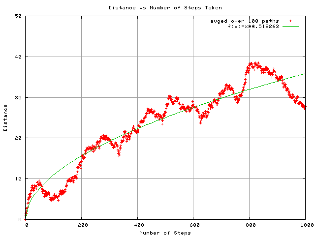
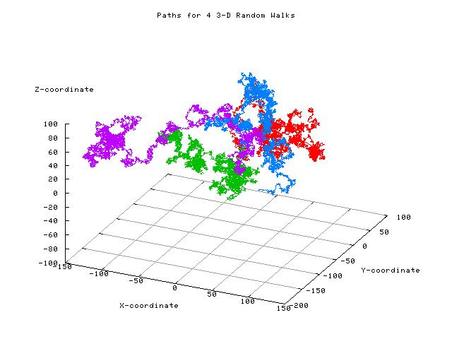
FIG5: Several 3D paths each consisting of 10k steps.
FIG4: Plot of D versus N for a paths with 1000 steps, where the number of paths averaged over was 4. D was fit as a function of N with equation: D=N^(.518).
B. 3D Path
FIG5: Several 3D paths each consisting of 10k steps.
The program for 3D
paths was run for paths with 10k steps. Four specific paths are
plotted in FIG5. D versus N when averaged over 100 paths is
plotted in FIG6. From the fit to the graph, p=0.529.
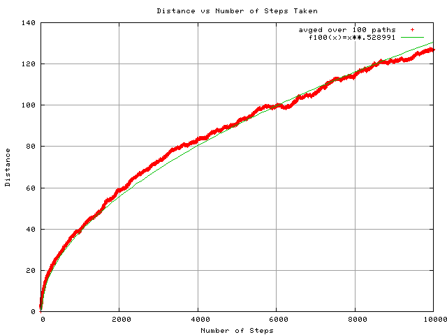
FIG6: D versus N for a 3D path of 10k steps. D is fitted as a function of N: D=N^(.529).
3. Conclusions
When walking a path, the average distance, D, is a function of the number of steps taken, N. The relationship is given by D=N^(p), where p is theoretically 0.5. In the 2D case, as the number of paths which are averaged to find D is increased, p (as determined by a fitting of the data) seems to approach the theoretical value. For only 10 paths p=0.492 as opposed to 100 paths, p=0.495, which is closer to 0.5. This makes sense because the randomness becomes averaged out as more paths are taken into account. This can also be seen graphically in FIG2. The case with 10 paths (blue) is more noisy when compare to the case with 100 paths (red). The case with only 4 paths each of 1000 steps (FIG4) has p=0.518. This is even further from the theoretical value than the cases with 10k steps per path. This may be due to lower statistics (less steps and less paths). Also, when the final coordinates (in x-y space) are plotted for the final position of several 10k step paths, a somewhat circular distribution is expected. The final positions should be centered about the origin. This is roughly observed in FIG3. The 3D random walk
shows p=0.529 (FIG6).
[1] R. H. Landau & M. J. Paez, Computational Physics, Problem Solving with Computers, (Wiley: New York) 1997.
[2] P. W. Gorham, http://www.phys.hawaii.edu/~gorham/P305/RandomWalks.html.
4.
References
[1] R. H. Landau & M. J. Paez, Computational Physics, Problem Solving with Computers, (Wiley: New York) 1997.
[2] P. W. Gorham, http://www.phys.hawaii.edu/~gorham/P305/RandomWalks.html.