Aaron Koga
Physics 305
6 March 2007
Physics 305
6 March 2007
1. Introduction
In a Poisson Process, the probability of an event occurring in a time interval, k, given about a known mean is given by:
 (1) [1].
Poisson Processes are random sequences
of events whose probabilities are distributed evenly in time or
space. One example of this, studied in this lab, is the number of
cars passing a certain point in a given period of time, where is
probability of a car passing the point is uniform throughout time.
One way to generate a probability distribution, f(x), such as the poisson distribution is to use the Von Neumann method. In this method, numbers that bound the distribution from above (Ymax), below (Ymin), right (Xmax), and left (Xmin) are chosen. A point, (x,y), is then randomly chosen (with uniform distribution in space) where Xmin<x<Xmax and Ymin<y<Ymax. Using only the points where y<f(x), a list of x is made. Using this list, the frequency of x versus x is plotted. This plot should follow f(x).
The amount of radioactive material left as it decays is exponential and given by:
 (2),
(2),
One way to generate a probability distribution, f(x), such as the poisson distribution is to use the Von Neumann method. In this method, numbers that bound the distribution from above (Ymax), below (Ymin), right (Xmax), and left (Xmin) are chosen. A point, (x,y), is then randomly chosen (with uniform distribution in space) where Xmin<x<Xmax and Ymin<y<Ymax. Using only the points where y<f(x), a list of x is made. Using this list, the frequency of x versus x is plotted. This plot should follow f(x).
The amount of radioactive material left as it decays is exponential and given by:
(2),where N(0) is the initial amount of
material and T is the lifetime of the material. Taking the
derivative of (2), the decay of a radioactive material is given by:
 (3).
(3).
This describes is the decay of carbon-14, carbon-11, and
carbon-10. The lifetime of C14, C11, and C10 are 5730 years, 1221
seconds, and 19.25 seconds respectively. Because of the long
lifetime of C14, carbon dating measures the age of a material by
finding the decay rate of C14 in that material. By comparing the
current decay rate to the original decay rate (15.0 decays/s/g), the
age can be found by using (3).
(3).2. Counting Cars
A C Program, cars.c, was written to simulate the arrival of cars
at a certain point. This simulated data was used to calculate the
rate of cars per minute passing the point. The arrival of cars is
simulated by using drand48(). The probability of a car passing
the point, prob, was assigned to be 0.1 (in a second) and the time
resolution, tInterval, was 0.01 seconds. Using drand48(), a
number between 0 and 1 was generated. The generated number was
then tested to see if it was below .001 (prob*tInterval). If the
number was below .001, then a car passed the point; if the number was
above .001, then no car had arrived. This testing of the
generated number enforced the probability of 0.1 for the arrival of
cars.
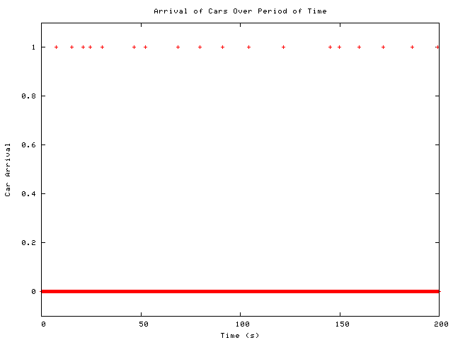
FIG1: Arrival of cars over a period of time (0-200 seconds), where 1 signifies that a car has arrived and 0 signifies that there is no car.
FIG1 shows the arrival of cars generated
using the method with drand48() over a 200 second window.
The data collected was then separated into 1 minute intervals and the rate of cars passing the point per minute was calculated. This is shown in FIG2.
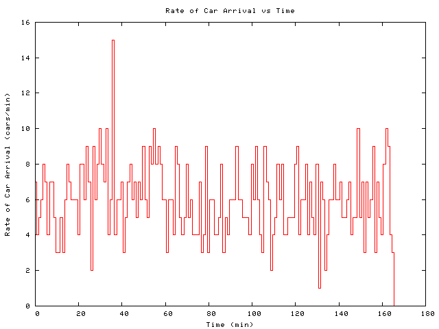
The data collected was then separated into 1 minute intervals and the rate of cars passing the point per minute was calculated. This is shown in FIG2.
FIG2: Rate of cars passing the point (cars/min) over a 166 minute window.
The data for the rate
of cars passing the point was then binned and a histogram was
plotted. The number of times a particular rate was observed
(counts) versus the rate (cars/min passing the point) is plotted in
FIG3. The data theoretically follows the poisson
distribution. Fitting the data yielded a mean value of
6.07+/-0.21 for the rate of cars/min. This is in line with the
settings used to generate the data using drand48(). The
probability of a car passing the point in a second was 0.1. Thus,
the rate of cars/min is 60*0.1=6.
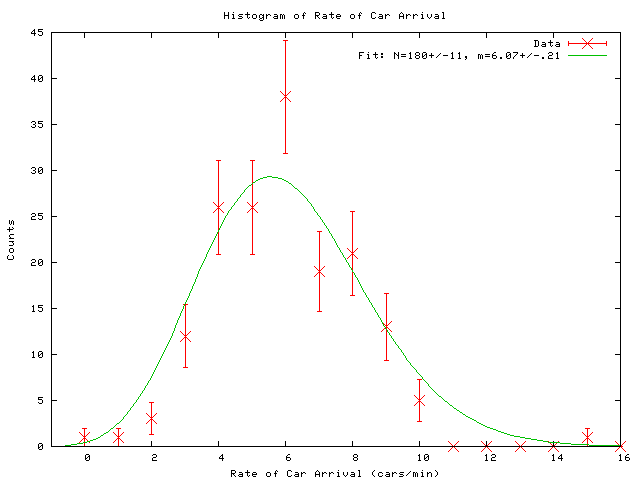
FIG3: Histogram of the rate of cars (cars/min) passing the point. Fitting the data to the poisson distribution gave a mean of 6.07+/-0.21.
3. Carbon Decay
A C Program, decay.c (shown in Appendix A), was written to
simulate the decay of C11 and C10 in a material. The program
takes command line inputs to define the number of atoms of C12, C11 and
C10 for a material to start with. The heart of
this program uses drand48() (in a way similar to that in which it
was used above) to
generate numbers to simulate the decay of an atom of carbon. If
drand48() produces a number that signals that a decay has occurred,
then the decayed atom is removed from the material and only the
remaining C11 or C10 atoms are able to decay. The time resolution
was set to 0.1 seconds. The decays were then used to find the
decay rate over a time interval of 10 seconds. The rate of decay
in a sample containing C11 and C10 with the initial amounts set to 1225
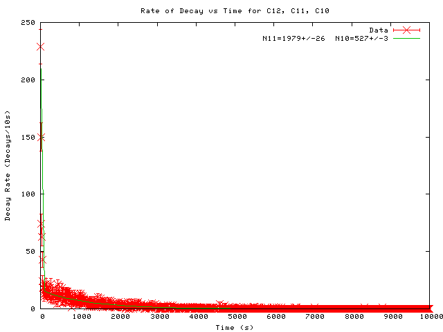
atoms each. The data, plotted in FIG4, shows that the initial
amount of C11, N11=1205+/-23 and C10, N10=1256+/-3 are close to the
initial values.
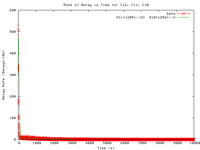
FIG4: Plot of decay rate for a sample with C11 and C10 fitted to N11/1221*exp(-t/1221)+N10/19.25*exp(-t/19.25).
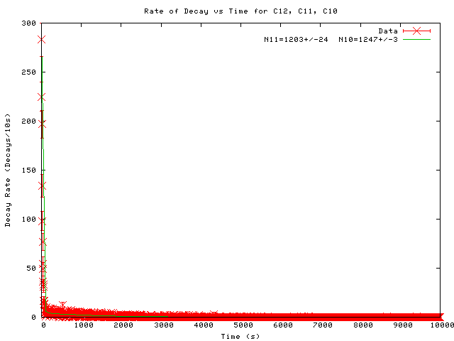
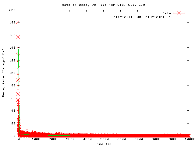
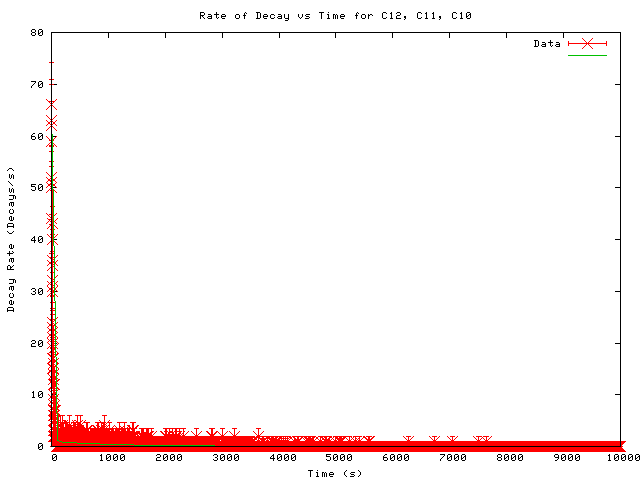
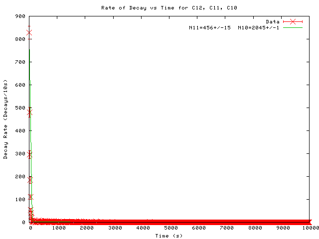
The rate of decay was simulated
using different initial amounts of C11 and C10. Different time
intervals over which the rate of decay was calculated were also
simulated. The data, summarized in Table1, suggests that as the
time interval is decreased N11 and N10 get closer to the initially set
values. Also, it seems as if the minimum number of atoms needed
to get a good fit to the data is 500.
Table1: Summary of fitted versus set N11 and N10.
N11 Set
(atoms)
N10 Set
(atoms)
Time
Interval (s)
N11 Found
(atoms)
N11 Error
(atoms)
N10 Found
(atoms)
N10 Error
(atoms)
Link to Plot
Table1: Summary of fitted versus set N11 and N10.
4. C14 Dating
A C Program, carbon.c
(shown in Appendix B), was written to
simulate the decay of C14 in different materials. This program
uses the Von Neumann method to generate the decay rate of C14
atoms. Because the lifetime of C14 is long, the decay rate over a
few hours can be approximated as constant and given by the poisson
distribution. Thus, the Von Neumann method was used to generate a
poisson distribution in the function get_xvalue(). Using this
function, the program generates an array of decay rates (decays/min),
which are binned and used to create a histogram.
The C14 decay of a 6 gram bone sample estimated to be 21,600 years old was simulated. The decay rate was measured for 12 hours (720 min). FIG5 shows the decay rate as a function of time. FIG6 shows a histogram of the decay rate fitted to the poisson equation. This gave the average decay rate as 6.29+/-0.06. And thus the age as 15246+/-55 years.
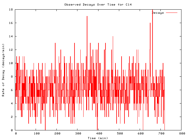
FIG5: Observed decay rate as a function of time for a 6 gram
bone.
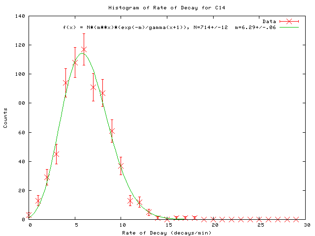
FIG6: Histogram of the decay rate of a 6 gram bone. Average
decays/min was found to be 6.29+/-0.06.
The C14 decay of a 6 gram bone sample estimated to be 21,600 years old was simulated. The decay rate was measured for 12 hours (720 min). FIG5 shows the decay rate as a function of time. FIG6 shows a histogram of the decay rate fitted to the poisson equation. This gave the average decay rate as 6.29+/-0.06. And thus the age as 15246+/-55 years.
FIG5: Observed decay rate as a function of time for a 6 gram
bone.
FIG6: Histogram of the decay rate of a 6 gram bone. Average
decays/min was found to be 6.29+/-0.06.
Similar tests were
performed for a linen with 0.2 g of C14 that was 1975 years old, the
same linen that was 700 years old, and 10 mg of C14 from a hair sample
known to be 4700 years old. The results are summarized in FIG7-12
and Table2.
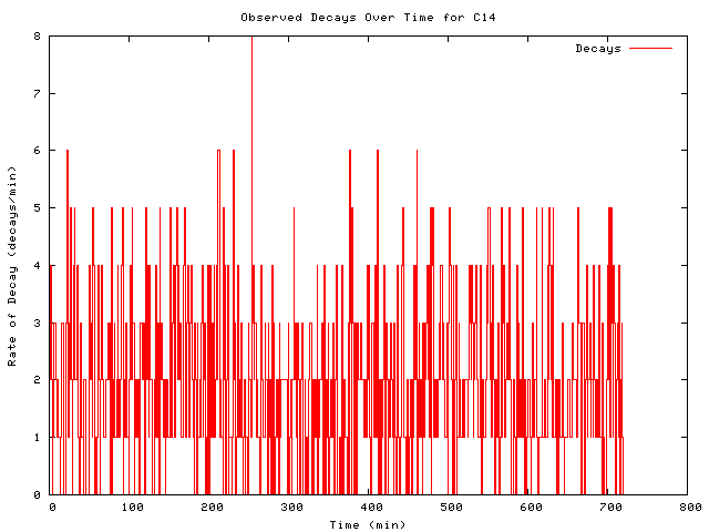
FIG7: Observed decay rate as a function of time for a 1975 year old
linen
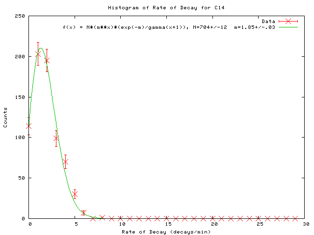
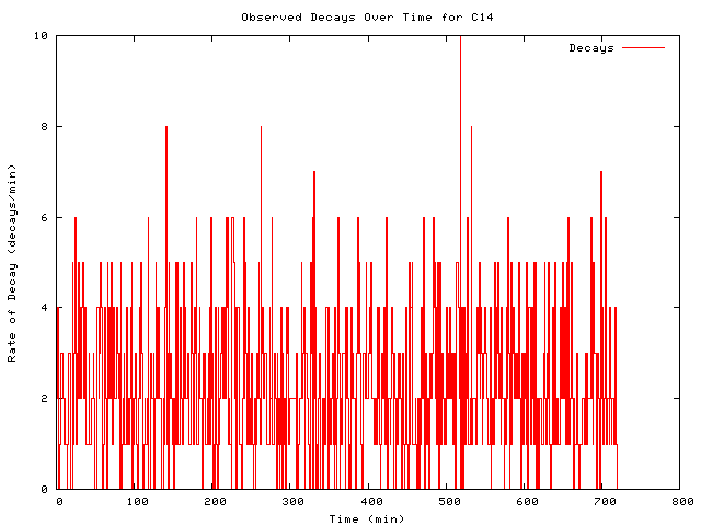
FIG9: Observed decay rate as a function of time for a 700 year old
linen
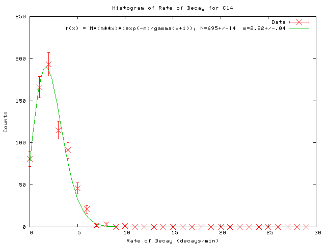
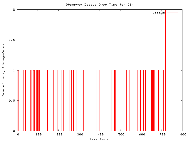
FIG11: Observed decay rate as a function of time for a hair
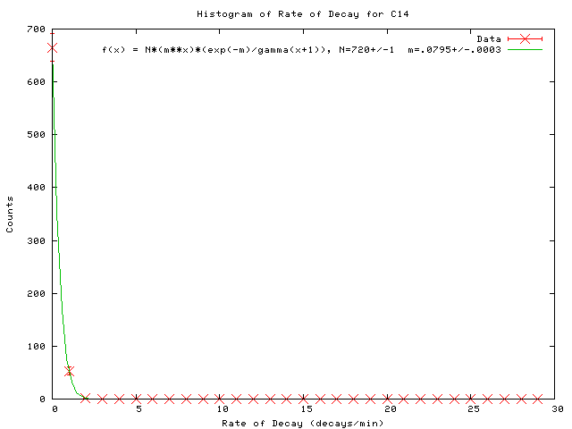
FIG7: Observed decay rate as a function of time for a 1975 year old
linen
FIG8: Histogram of the decay rate of a 1975 year old linen. Average decays/min was found to be 1.85+/-0.03.
FIG9: Observed decay rate as a function of time for a 700 year old
linen
FIG10:Histogram of the decay rate of a 700 year old linen. Average decays/min was found to be 2.22+/-0.04.
FIG11: Observed decay rate as a function of time for a hair
FIG12:Histogram of the decay rate of a hair. Average decays/min was found to be 0.0795+/-0.0003.
Material
Theoretical
Age (years)
Average
Decay Rate (decays/min)
Error in
Decay Rate
Measured Age
(years)
Duration of
Measurement (hours)
bone with 6g
carbon
21600
6.29
0.06
15246+/-55
12
linen with
.2g carbon
1975
1.83
0.03
2770+/-62
12
linen with
.2g carbon
700
2.22
0.04
1725+/-100
12
hair with
10mg carbon
4700
0.0795
0.0003
3638+/-20
12
Table2: Table summarizing simulated carbon dating, measuring
the sample for 12 hours.
5. Conclusion
In section2, the
value for the mean rate of arrival of cars given from fitting the
simulated data to a poisson distribution, 6.07+/-0.21, agreed with the
set value of 6. In the simulation of C11 and C10 decay, although
the simulation became better as the time interval (used to calculate
the rate of decay) decreased, this effect was not very
significant. Also, it seemed as if the minimum number of atoms
needed to create a reasonable simulation was 500 for both C11 and
C10. The measured ages from the simulation of C14 decay in
section4 did not agree with the theoretically given/set ages.
This is probably due to the fact that the decay of C14 from the samples
was only measured for 12 hours in the simulation. Measuring the
decay rate for a longer period of time might improve measured ages.
6.
References
[1] P. W. Gorham, http://www.phys.hawaii.edu/~gorham/P305/MCfitting1.html
[2] P. W. Gorham, http://www.phys.hawaii.edu/~gorham/P305/IsotopeDecay.html
[3] R. H. Landau & M. J. Paez, Computational Physics, Problem Solving with Computers, (Wiley: New York) 1997.