Aaron Koga
Physics 305
20 Feb 2007
Physics 305
20 Feb 2007
1. Introduction
Even if an analytic integral exists, integration in high-dimensional systems can be difficult. One method for easily calculating integrals, even in a large number of dimensions, is Monte Carlo Integration. This method uses uniform randomly generated numbers to determine an integral. For example, suppose we want to find the area of a circle. We can then define another area, a box, that completely encloses the circle. We then pick points within the box that are uniformly and randomly distributed. After picking some points, we can find the ratio of the area of the circle to the area of the box by
 (1),
(1),where Ncircle is the number
of points that fell within the circle and Ntotal is the
number of points picked. From this ratio the area of the circle
can be found by
 (2).
(2).
(2).This analysis can easily be extended to
higher dimensions with computers.
Because this is a statistical method, the error in the calculated integral should decrease by n-1/2 [1].
Because this is a statistical method, the error in the calculated integral should decrease by n-1/2 [1].
2. Volume of a Sphere
A. C Program to Find the Volume of a Sphere
A C Program (pond2.c
[2]) was modified and used to calculate the volume of a sphere by Monte
Carlo integration. The program, pond3.c is
shown in the Appendix. pond3.c uses the
function drand48() to generate random coordinates within a 3D cube to
find the volume of an inscribed sphere. In the program, the
radius of the sphere is 1 and the length of a side of the cube is
2. The number generated by drand48(), which is in the range
(0,1), is centered about zero and allowed to be in the range (-1,1) by
the formula:
 (3).
(3).
(3).One of these random numbers is generated
for each coordinate and the distance from the origin is used to
determine if the point in 3D space falls within the sphere. The
volume is then found by the method mentioned above and the data for the
calculated volume and the error in it are printed to a file.
B. Results for the Volume of a Sphere
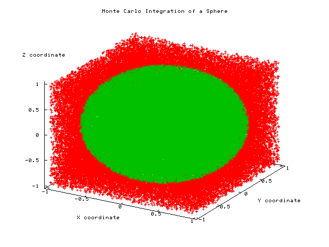
FIG1: Plot of the points selected in 3D space, where the points falling within the sphere are plotted in green and the points falling outside of the sphere are plotted in red.
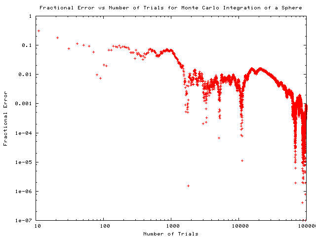
FIG2: Plot of the Fractional Error in calculating the volume of a sphere versus the number of points selected (Number of Trials).
The program pond3.c
was used to find the volume of a sphere. The points selected in
3D space are shown in FIG1. The fractional error is shown in FIG2
as a function of the number of points selected. Although there
are fluctuations, the error generally decreases as the number of
selected points increases.
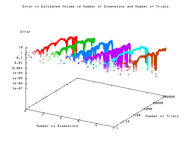
FIG7: Plot of the fractional error as a function of the
number of dimensions and number of points selected.
3. Volume of a Hypersphere
A. C Program to Find the Volume of a Hypersphere
A C program (hypersphereMC.c
[2]) was completed and used to find the volume of a hypersphere of up
to 10 dimensions by Monte Carlo integration. hypersphereMC.c is
shown in the Appendix.
This program uses the same mechanism as pond3.c to select points in an
N-D space. Also like pond3.c, each hypersphere has a radius of 1
and each hypercube has sides of length 2. However, the
hypersphereMC.c selects points for dimensions up to 10, printing the
volume and fractional error to a file for all dimensions from 1 to
10. The program also accepts as a command line input the number
of dimensions and the number of points taken in that dimensions.
These numbers, specified by the user, are printed to the screen for
easy viewing.
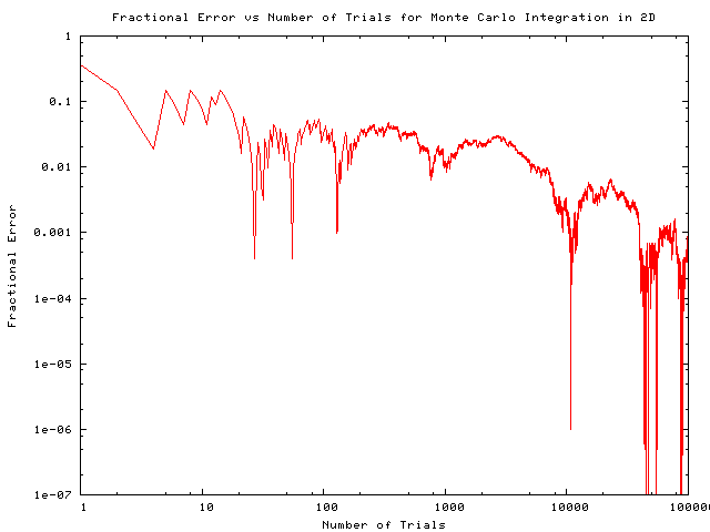
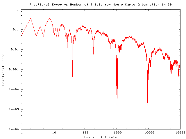
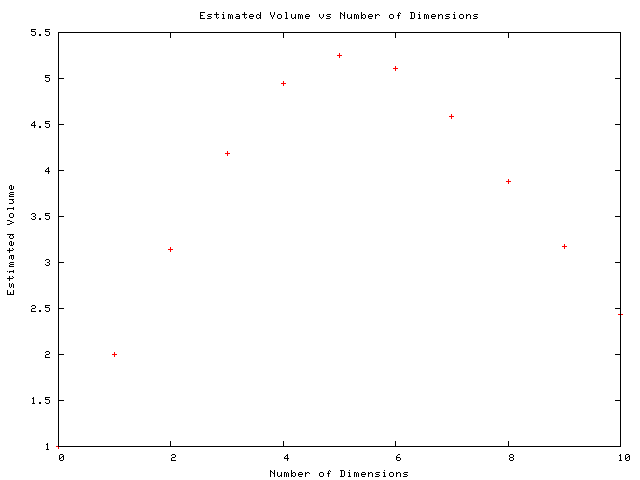
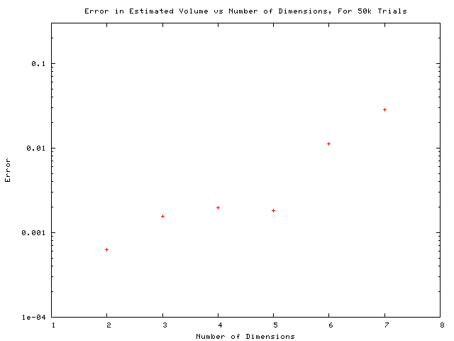
FIG6: Plot of the fractional error in the calculation of the
volume of a hypersphere vs number of dimensions using 50k selected
points.
B. Results for the Volume of a Hypersphere
The program
hypersphereMC.c was first used to find the area of a 2D circle and the
volume of a 3D sphere. The fractional error is shown in FIG3 and
FIG4 as a function of the number of points selected for both the 2D and
3D cases. As can be seen from the graphs, the error in
calculating the area/volume of a circle/sphere generally decrease as
the number of selected points used in the calculation increase.
FIG3: Plot of the fractional error vs number of selected points when using the program hypersphereMC.c to find the area of a circle (2D).
FIG4: Plot of the fractional error vs number of selected points when using the program hypersphereMC.c to find the volume of a 3D sphere.
Volume of
hyperspheres in higher dimensions were then examined using
hypersphereMC.c. FIG5 shows a plot of the estimated volume of a
hypersphere as a function of its number of dimensions. These
numbers were generated using 50k points to calculate the volume of each
hypersphere. FIG6 shows a plot of the fractional error in the
estimated volume as a function of the number of dimensions. These
calculations were made using 50k points to calculate the volume of each
hypersphere. The graph shows that the error generally increases
as the number of dimensions increase.
FIG5: Plot of the estimated volume of a hypersphere vs the number of dimensions using 50k points per dimension.
FIG6: Plot of the fractional error in the calculation of the
volume of a hypersphere vs number of dimensions using 50k selected
points.
FIG7 shows a plot of
the fractional error (in the calculation of the volume of a
hypersphere) as a function of the number of dimensions and number of
points selected to calculate the volume of the hypersphere. The
general trend is that as the number of selected points increases in a
given dimension, the error decreases.
FIG7: Plot of the fractional error as a function of the
number of dimensions and number of points selected.
3. Conclusions
According to Landau and Paez, the fractional error due to Monte Carlo integration should decrease as n-1/2 [1]. From FIG2-4, it seems that the error generally decreases with the number of selected points. This general trend can also be seen for a given dimension in FIG7. However, because of the fluctuations it is hard to determine if it decreases as n-1/2. Because the points are randomly generated, it is not too surprising that there are fluctuations in the error.For a fixed number of points (50k in this lab), FIG6 shows that the error increases with the number of dimensions. This is expected because as the number of dimensions increases, the number of points is distributed over a larger number of dimensions.
When examining the volume of a hypersphere as a function of the number of dimensions (FIG5), it looks like the volume increases until 5 dimensions, where it starts to decrease. This might seem surprising, but can be expected for this case, where the radius of all hyperspheres was 1. The analytic volume of a hypersphere in N-dimensions goes as RN, where R is the radius [3]. However, because the radius here was always 1, this dependency did not play a role in the estimated volumes for this lab. Thus, the plot shown in FIG5 is actually an estimation of the coefficients used in the calculation of the N-D hyperspheres (that is C in the expression: Volume=C*RN, where C is a constant).
4.
References
[1] R. H. Landau & M. J. Paez, Computational Physics, Problem Solving with Computers, (Wiley: New York) 1997.
[2] P. W. Gorham, http://www.phys.hawaii.edu/~gorham/P305/MonteCarlo1.
[3] K. Enevoldsen, http://thinkzone.wlonk.com/MathFun/Dimens.htm.