Aaron Koga
Physics 305
20 March 2007
Physics 305
20 March 2007
1. Introduction
Solving differential
equations is very important in physics. However, many
differential equations cannot be solved analytically. Thus, they
must be solved numerically. One method for doing this is the
Euler Method. Basically, this method uses the slope of a function
to integrate a differential equation at fixed intervals. That is,
for an equation
2. Simple Harmonic Oscillator
A. Euler
dy/dt=f(t,y)
(1),
y(t+dt)=y(t)+dt*f(t,y) (2).
y(t+dt)=y(t)+dt*f(t,y) (2).
For example, consider a simple harmonic
oscillator where F=-kx. Then,
F = - k x = m dv/dt, so
dv/dt = - kx/m (3)
dx/dt = v (4) .
dv/dt = - kx/m (3)
dx/dt = v (4) .
Although this is a simple method, for
finite dt it accumulates error. [1]
Another numerical method of solving differential equations is the Runge Kutta Method. There are both second order (RK2) and fourth order (RK4) methods of approximation. The RK2 method for a function of the form (1) is:
Another numerical method of solving differential equations is the Runge Kutta Method. There are both second order (RK2) and fourth order (RK4) methods of approximation. The RK2 method for a function of the form (1) is:
y(t + dt) = y(t)
+ k2
(5)
k2 = dt * f( t+dt/2 , y(t)+ k1/2 )
k1 = dt * f( t , y(t) ).
k2 = dt * f( t+dt/2 , y(t)+ k1/2 )
k1 = dt * f( t , y(t) ).
For the simple harmonic oscillator this
method can be used to solve equations (3) and (4). The RK4 method
for an equation of the form (1) is:
y(t+dt)
= y(t) + 1/6 * (k1
+
2k2 + 2k3
+ k4) (6)
k1 = dt * f(t,y)
k2 = dt * f(t+dt/2, y(t)+k1/2)
k3 = dt * f(t+dt/2, y(t) + k2/2)
k4 = dt * f(t+dt, y(t)+k3)
k1 = dt * f(t,y)
k2 = dt * f(t+dt/2, y(t)+k1/2)
k3 = dt * f(t+dt/2, y(t) + k2/2)
k4 = dt * f(t+dt, y(t)+k3)
and can be used in the same fashion as
the RK2 method. [2]
2. Simple Harmonic Oscillator
A. Euler
A C Program, harmosc1.c (Appendix A), was
written and used to solve the simple harmonic oscillator using the
Euler Method. This program was used to simulate an oscillator
with parameters k=m=1, initial velocity (v(0)), and starting position
(x(0)) of zero for different values of dt. Using dt=1ms, the
program was run and the results are shown in FIG1. Theoretically
a harmonic oscillator has a period of 2(pi)sqrt(k/m), which in this
case is 6.28s. The period as measured by eye from FIG1 is about
6s.
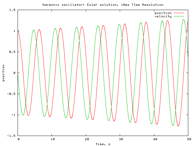
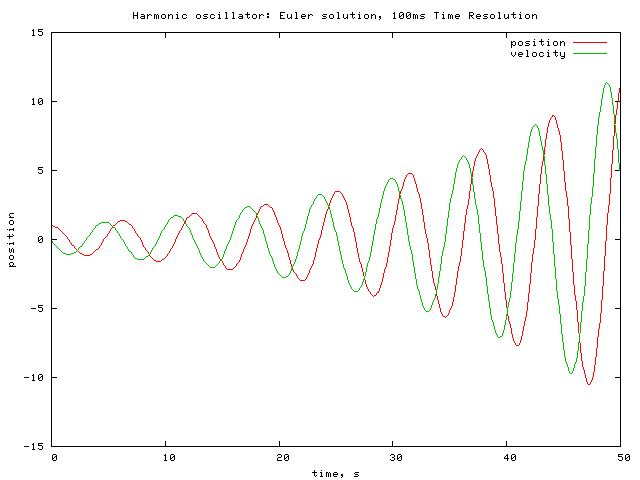
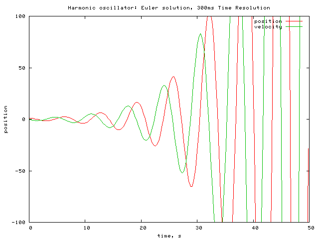
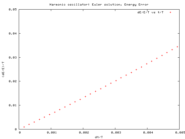
The value of dt was changed to 10ms, 100ms, and 300ms. The output from the program is shown in FIG2-4. As can be seen from the graphs, the oscillations for x and v become bigger with time. This means that the energy is not constant and increases with time. A graph of the fractional increase in energy per period (T) as a function of the fraction dt/T is shown in FIG5. The error in energy increases as dt increases. This is not surprising because as the Euler Method does not account for changes in the slope of the function between intervals of dt. The bigger dt becomes, the more the slope of the function between intervals is left unaccounted and the error in the energy increases.
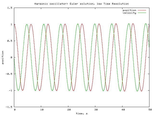
FIG1: Simulation of harmonic oscillator using Euler Method
with: k=m=x(0)=1, v(0)=0, dt=1ms.
The value of dt was changed to 10ms, 100ms, and 300ms. The output from the program is shown in FIG2-4. As can be seen from the graphs, the oscillations for x and v become bigger with time. This means that the energy is not constant and increases with time. A graph of the fractional increase in energy per period (T) as a function of the fraction dt/T is shown in FIG5. The error in energy increases as dt increases. This is not surprising because as the Euler Method does not account for changes in the slope of the function between intervals of dt. The bigger dt becomes, the more the slope of the function between intervals is left unaccounted and the error in the energy increases.
FIG1: Simulation of harmonic oscillator using Euler Method
with: k=m=x(0)=1, v(0)=0, dt=1ms.
FIG2: Simulation of harmonic oscillator using Euler Method with: k=m=x(0)=1, v(0)=0, dt=10ms.
FIG3: Simulation of harmonic oscillator using Euler Method with: k=m=x(0)=1, v(0)=0, dt=100ms.
FIG4: Simulation of harmonic oscillator using Euler Method with: k=m=x(0)=1, v(0)=0, dt=300ms.
FIG5: Fractional error in energy per period as a function of dt/T for the Euler solution to the harmonic oscillator.
B. RK2 & RK4
A C Program, harmoscRK.c (Appendix B)
was also written to simulate the harmonic oscillator using the RK2 and
RK4 methods. This program uses the methods outlined by equations
(5) and (6) to calculate the RK2 and RK4 approximations for the
oscillator. Functions FRK2 and FRK4, which in turn
call other functions for dx/dt and dv/dt,
are used to make these approximations . Output from the program for the RK2 solution
and RK4 solution is plotted in FIG6 and FIG7 respectively. Also,
the fractional energy error per period is plotted as a function of dt/T
for RK2, RK4 and Euler Methods in FIG8. As FIG8 shows, the RK2
and RK4 methods, though not really different from each other, provide
better approximations (less energy error) than the Euler Method.
While the RK2 and RK4 methods do not fully account for changes in slope
of a function, these methods attempt to do so. This makes them
better approximations than the Euler Method. The Euler Method has
a 1% energy error for dt~.15% of a period. On the other hand, the
RK2 and RK4 methods give a 1% energy error when dt~.3% of a
period.
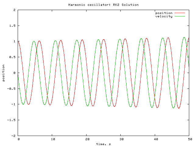
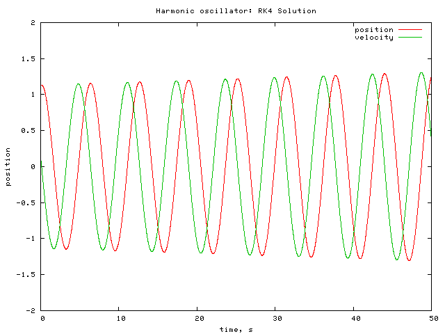
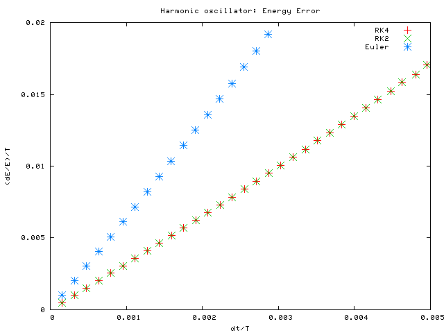
FIG6: Simulation of harmonic oscillator using RK2 Method with: k=m=x(0)=1, v(0)=0, dt=1ms.
FIG7: Simulation of harmonic oscillator using RK4 Method with: k=m=x(0)=1, v(0)=0, dt=1ms.
FIG8: Comparison of fractional error in energy per period as a function of dt/T for the different methods of solving the harmonic oscillator.
3. Pendulum
A pendulum is subject
to:
 (7).
(7).
(7).Like the harmonic oscillator, this can
be broken into two equations:
 (8)
(8)
 (9).
(9).
Using equations (8) and (9) to make calculations of a pendulum, a C Program, pendulum.c, was written. This program used the same method as harmosc1.c and harmoscRK.c to approximate a pendulum based on the Euler and RK2 solutions. While the same method was used, the functions for dx/dt and dv/dt in the harmonic oscillator were replaced (Appendix D).
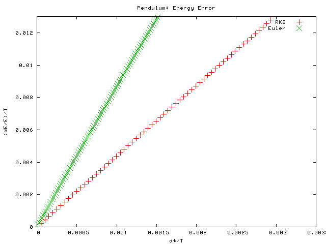
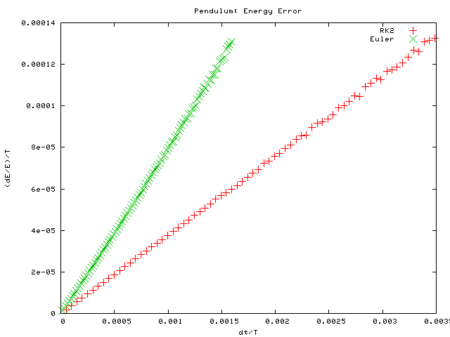
The program was run using the parameters dt=.1ms, g=9.8, and L=1 with an initial angle of 166 degrees and initial angular velocity of 0 degrees. The output for the Euler and RK2 Methods are shown in FIG9 and FIG10 respectively. The fractional energy error as a function of dt/T is shown in FIG11. Once again, the energy error of the RK2 method is smaller than that of the Euler Method. The initial angle was then changed from 166 degrees to 5 degrees. The fractional energy error as a function of dt/T for a 5 degree initial angle is plotted in FIG12. When comparing FIG11 and FIG12, it seems that the error is larger for larger initial angles. At small angles, it is known that the pendulum approaches the sinusoidal behavior of a harmonic oscillator. However, this is not the case for larger angles, where the behavior of the pendulum is not as "nice." This is reflected in the difference between FIG11 and FIG12.
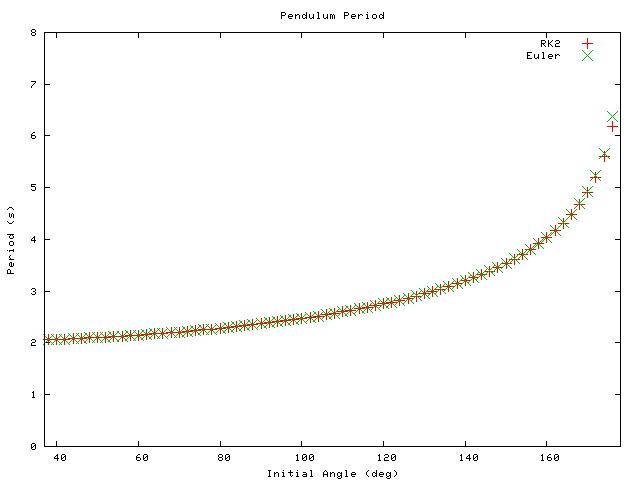
FIG13 shows that the period of the pendulum increases with the initial angle (for both the Euler and RK2 methods). This is reasonable because at large angles, the pendulum has farther to swing to complete a period.
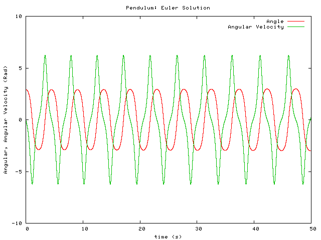
FIG9: Simulation of a pendulum using the Euler Method with g=9.8,
L=1, initial angle=166 degrees, initial angular velocity=0.
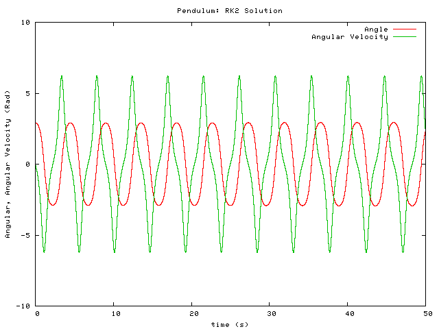
FIG10: Simulation of a pendulum using the RK2 method with g=9.8,
L=1, initial angle=166 degrees, initial angular velocity=0.
(8)(9).Using equations (8) and (9) to make calculations of a pendulum, a C Program, pendulum.c, was written. This program used the same method as harmosc1.c and harmoscRK.c to approximate a pendulum based on the Euler and RK2 solutions. While the same method was used, the functions for dx/dt and dv/dt in the harmonic oscillator were replaced (Appendix D).
The program was run using the parameters dt=.1ms, g=9.8, and L=1 with an initial angle of 166 degrees and initial angular velocity of 0 degrees. The output for the Euler and RK2 Methods are shown in FIG9 and FIG10 respectively. The fractional energy error as a function of dt/T is shown in FIG11. Once again, the energy error of the RK2 method is smaller than that of the Euler Method. The initial angle was then changed from 166 degrees to 5 degrees. The fractional energy error as a function of dt/T for a 5 degree initial angle is plotted in FIG12. When comparing FIG11 and FIG12, it seems that the error is larger for larger initial angles. At small angles, it is known that the pendulum approaches the sinusoidal behavior of a harmonic oscillator. However, this is not the case for larger angles, where the behavior of the pendulum is not as "nice." This is reflected in the difference between FIG11 and FIG12.
FIG13 shows that the period of the pendulum increases with the initial angle (for both the Euler and RK2 methods). This is reasonable because at large angles, the pendulum has farther to swing to complete a period.
FIG9: Simulation of a pendulum using the Euler Method with g=9.8,
L=1, initial angle=166 degrees, initial angular velocity=0.
FIG10: Simulation of a pendulum using the RK2 method with g=9.8,
L=1, initial angle=166 degrees, initial angular velocity=0.
FIG11: Fractional energy error per period vs dt/T for a pendulum with initial angle=166 degrees.
FIG12: Fractional energy error per period vs dt/T for a pendulum with initial angle=5 degrees.
FIG13: Period of a pendulum vs initial angle.
4. Damped Harmonic Oscillator
A C Program, dampHarmosc.c, using the RK2 method was
written to simulate a damped harmonic oscillator. A damping force
of -bv was used. Using this damping factor, the equations for the
oscillator are:
F = - kx -bv = m dv/dt, so
dv/dt = (-kx -bv)/m (10)
dx/dt = v (11).
dv/dt = (-kx -bv)/m (10)
dx/dt = v (11).
The functions for dv/dt and dx/dt
were modified to fit equations (10) and (11).
Using k=m=x(0)=1, v(0)=0, dt=.1ms, and b=.15, the program was run and the output is shown in FIG14. To check the program, b was set to 0, which should produce the same output as a simple harmonic oscillator. The output for b=0, graphed in FIG15, looks like that of a simple harmonic oscillator.
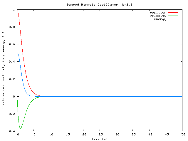
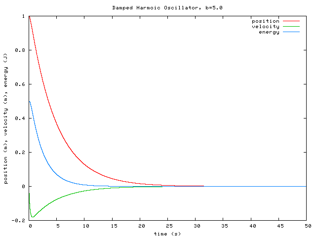
Critical damping for a harmonic oscillator is given by b/2m=k/m. For the parameters given above, this means that b=2 for critical damping. The output of the program with b=2 is shown in FIG16. This definitely looks like a critically damped oscillator. If b/2m>k/m, then the oscillator is over damped. This case was simulated for b=5, with the output of the program graphed in FIG17. The settling time of the over damped oscillator is greater than the critically damped oscillator.
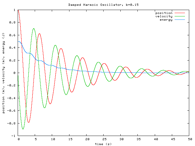
FIG14: Simulation of damped harmonic oscillator with the RK2 method
using b=.15.
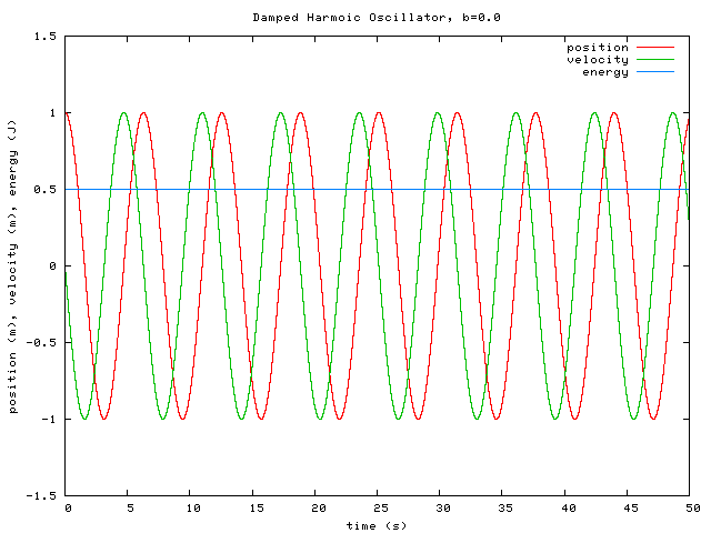
Using k=m=x(0)=1, v(0)=0, dt=.1ms, and b=.15, the program was run and the output is shown in FIG14. To check the program, b was set to 0, which should produce the same output as a simple harmonic oscillator. The output for b=0, graphed in FIG15, looks like that of a simple harmonic oscillator.
Critical damping for a harmonic oscillator is given by b/2m=k/m. For the parameters given above, this means that b=2 for critical damping. The output of the program with b=2 is shown in FIG16. This definitely looks like a critically damped oscillator. If b/2m>k/m, then the oscillator is over damped. This case was simulated for b=5, with the output of the program graphed in FIG17. The settling time of the over damped oscillator is greater than the critically damped oscillator.
FIG14: Simulation of damped harmonic oscillator with the RK2 method
using b=.15.
FIG15: Simulation of damped harmonic oscillator with the RK2 method using b=0.
FIG16: Simulation of damped harmonic oscillator with the RK2 method using b=2.
FIG17: Simulation of damped harmonic oscillator with the RK2 method using b=5.
5. References
[1] P. W. Gorham, http://www.phys.hawaii.edu/~gorham/P305/DiffEq1.html
[2] P. W. Gorham, http://www.phys.hawaii.edu/~gorham/P305/DiffEq2.html
[3] R. H. Landau & M. J. Paez, Computational Physics, Problem Solving with Computers, (Wiley: New York) 1997.