Abstract:
This paper examines the risk-reward trade-off in the portfolio of an individual investor of Vanguard funds. The investor must pay for living expenses from the investments and conform to the minimum investment amount at Vanguard. The efficiency frontier is found for two situations: one where the investor makes investments and payments in dollars, and one where the investor makes investments in dollars and payments in yen.
FINAL PROJECT - PORTFOLIO OPTIMIZATION FOR A SMALL INVESTOR AT VANGUARD WITH REQUIRED WITHDRAWALS
Aaron Koga
Econ 429
3 May 2007
Introduction
A common question among investors is how and where to put their money in order to obtain maximum returns subject to certain requirements on risk and diversity. Often times, people not only want to earn a return on their money, but also want to use a portion of it for consumption. For example, retirees need to use their investments for personal consumption without totally depleting their investments. For most people, effective investing involves putting money into a combination of stocks, bonds, and money market funds or bank accounts. One convenient way to make and manage these different types of investments is with an investment company. One such company is Vanguard.
Vanguard is known for their low-cost, passively managed funds, which offer a wide array of investment options. Each fund has an associated minimum investment amount and annual fees.
The Situation and Problem
Suppose an investor named Bob, who is currently working a modest job,
is planning to go back to school to further his education in graduate school.
He currently has ![]() 50,000 in savings, which he must use to cover his expenses for the next
few years.
Fortunately, he has received a small fellowship to support his graduate studies and thus anticipates
that he will only need
50,000 in savings, which he must use to cover his expenses for the next
few years.
Fortunately, he has received a small fellowship to support his graduate studies and thus anticipates
that he will only need ![]() 500 a month from his savings.
Bob has heard good things about Vanguard and wants to invest his
500 a month from his savings.
Bob has heard good things about Vanguard and wants to invest his ![]() 50,000 among a few funds,
shown in TABLE I.
Because Bob is going to be a graduate student, he will not have much time to tend to his investments.
Therefore, he will only change his portfolio allocation once a quarter.
Because he wants diversity, Bob does not want more than
50,000 among a few funds,
shown in TABLE I.
Because Bob is going to be a graduate student, he will not have much time to tend to his investments.
Therefore, he will only change his portfolio allocation once a quarter.
Because he wants diversity, Bob does not want more than ![]() 15,000 in any one fund at any time.
Bob wants to know the trade-off between the variance of his portfolio (risk) and his ending balance
after one year of investment (reward).
15,000 in any one fund at any time.
Bob wants to know the trade-off between the variance of his portfolio (risk) and his ending balance
after one year of investment (reward).
Out of curiosity, Bob also wonders how an exchange rate would affect this optimization. If he were to study in Japan, his living expenses ($500/month) would be in yen. He wants to know if he could benefit from making smart decisions about when and how much money to exchange (from dollars to yen).
Formal Model, no Exchange Rate
To address Bob's fist question (the one without the exchange rate), the following non-linear model was developed and optimized.
Decision Variables
To allow quarterly changes to the portfolio, the decision variables were chosen as:
Definitions
The return and cost of fund
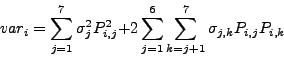
The variance in any quarter is
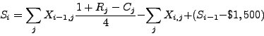
![]() represents money
reserved for consumption in a bank account.
This surplus is given by:
represents money
reserved for consumption in a bank account.
This surplus is given by:
Objective
To find the relationship between risk (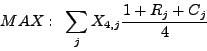
Constraints
The usual non-negativity constraint,was used. In addition, to provide the linking constraint and impose the minimum investment amount (
To impose the starting amount (![]() 50,000), the constraint
50,000), the constraint
was imposed. To satisfy the required withdrawals (
To trace out the efficiency frontier, a maximum value was set for the total variance.
Spreadsheet Implementation, no Exchange Rate
This non-linear problem was implemented and solved in an excel spreadsheet.
A screen capture of the spreadsheet is shown in FIG 3.
Some formulas from the spreadsheet are highlighted in TABLE II.
Excel's non-linear solver was used to maximize the ending balance for various
values of the maximum
![]() .
The results, plotted in FIG 1, show that the maximum ending balance
of $50,900 occurs with a
.
The results, plotted in FIG 1, show that the maximum ending balance
of $50,900 occurs with a
![]() of 2.7(10
of 2.7(10![]() ).
On the other hand, the minimum
).
On the other hand, the minimum
![]() of
2.5(10
of
2.5(10![]() ) is achieved at the cost of a $45,800 ending balance.
) is achieved at the cost of a $45,800 ending balance.
![\begin{figure}
\epsfxsize =3in
\epsfbox{dataNoExchange.eps}
%\includegraphics[width=9in, angle=90]{picNoExchange.eps}
\end{figure}](/wp-content/uploads/manual/econ429/img35.png)
Adding an Exchange Rate
The previous model assumes that Bob will be studying in the United States. However, if Bob were to study in Japan next year, he will be faced with living expenses in yen. Thus, he must take into account the dollar-yen exchange rate. Bob wants to know if he can save money by exchanging more dollars to yen at favorable exchange rates, rather than exchanging money without regard to the exchange rate. A few simple changes can be made to the previous non-linear model in order to answer this question.
Assume that the living expenses are now
178,410 yen/quarter (determined by the exchange rate on 4/7/07).
To pay for this, money can be exchanged from dollars to yen once a quarter at the exchange rates of
117.36, 113.87, 114.52, and 117.49 yen/$ ![]() .
.
Letting ![]() be the exchange rate in quarter
be the exchange rate in quarter ![]() ,
the equation governing the required withdrawals (EQ 10) becomes
,
the equation governing the required withdrawals (EQ 10) becomes
sets a maximum limit on how much money can be exchanged at one time. Because Bob is not trying to use yen as an alternative investment, there is no reason to exchange more than $6,000 (his approximate total living expenses for the year) at a time. See Appendix B for the full formulation of this model.
This model was solved using an excel spreadsheet (a screen shot is shown in FIG 4).
This spreadsheet was very similar to the one used to solve the model with no exchange rate.
Again, excel's non-linear solver was used to maximize the ending balance for various
values of the maximum
![]() .
.
First, the spreadsheet was solved with
![]() ; this simulated exchanging money without
regard to the exchange rate (a modification to EQ 12).
The spreadsheet was then solved with
; this simulated exchanging money without
regard to the exchange rate (a modification to EQ 12).
The spreadsheet was then solved with
![]() , simulating the exchange of money
at opportune times.
, simulating the exchange of money
at opportune times.
![\begin{figure}
\epsfxsize =3in
\epsfbox{dataExchange.eps}
%\includegraphics[width=9in, angle=90]{picNoExchange.eps}
\end{figure}](/wp-content/uploads/manual/econ429/img42.png)
The results, plotted in FIG 2, show that the difference between exchanging money at opportune times does not make a big difference in the ending balance after one year. For the exchange rate used here, the largest difference is less than $100 and most of the savings is below $20. The ending balance as a function of the total variance in this model with the exchange rate is very similar to the trade-off seen in the model without the exchange rate.
Summary of Results
For an investor putting money a small number of Vanguard funds
while using those funds to cover living expenses,
there is a wide range of possible trade-offs between risk and reward.
The ending balance after one year ranges from about $46,000 to almost $51,000.
The portfolio variance ranges over two orders of magnitude, from 2.5(10![]() to 2.7(10
to 2.7(10![]() ).
).
If the investor wishes to live in Japan, he
becomes subject to the fluctuating exchange rate.
Even if money is exchanged from dollars to yen at favorable exchange rates rather than
in regular amounts without regard for the exchange rate,
no more than $100 can be saved.
In fact, most savings is below $20.
While meager savings is the result for the case presented here,
it is possible that the savings can increase with different exchange rates (![]() ).
A more in-depth study using various exchange rates (perhaps generated by a monte carlo method)
would provide a better answer for possible savings.
).
A more in-depth study using various exchange rates (perhaps generated by a monte carlo method)
would provide a better answer for possible savings.
References
[1] Data for Vanguard funds can be found at: https://flagship.vanguard.com/VGApp/hnw/FundsByType
[2] Ragsdale, C. T. Spreadsheet Modeling and Decision Analysis, 5th Edition. Thomson, 2007.
[3] Data for exchange rate can be found at: http://www.oanda.com/convert/fxhistory
Appendix
Model for No Exchange Rate
LET:Total Variance=
![]() and
and ![]() is the variance of
is the variance of
a fund ![]() and
and ![]() is the covariance of funds
is the covariance of funds ![]() and
and ![]() .
.
![]() be the portion of total money in fund
be the portion of total money in fund ![]() in quarter
in quarter ![]() .
.
![]() be surplus money, not invested in any fund during
be surplus money, not invested in any fund during
quarter ![]() .
.
BY CHANGING:
![]() ,
, ![]()
MAX:
![]()
SUBJECT TO:
![]()
![]()
![]()
![]()
![]()
![]() , A is a number
, A is a number
Model with Exchange Rate
LET:Total Variance=
![]() and
and ![]() is the variance of
is the variance of
a fund ![]() and
and ![]() is the covariance of funds
is the covariance of funds ![]() and
and ![]() .
.
![]() be the portion of total money in fund
be the portion of total money in fund ![]() in quarter
in quarter ![]() .
.
![]() be surplus money, not invested in any fund during
be surplus money, not invested in any fund during
quarter ![]() .
.
![]() be the exchange rate in quarter
be the exchange rate in quarter ![]() .
.
BY CHANGING:
![]() ,
, ![]()
MAX:
![]()
SUBJECT TO:
![]()
![]()
![]()
![]()
![]()
![]() , A is a number
, A is a number
![]()
![\includegraphics[width=9.5in, angle=90]{picNoExchange.eps}](/wp-content/uploads/manual/econ429/img56.png)
|
![\includegraphics[width=9.5in, angle=90]{picExchange.eps}](/wp-content/uploads/manual/econ429/img58.png)